Conferences confine a paper to be at most X pages in length, where X is usually 7-10 pages. The need to communicate most of the important (theoretical and experimental) parts of my work in such a format means making sacrifices - this often ends in me removing text that aims to build intuitive reasoning behind the work.

While this is fine for reviewers, who are usually knowledgeable about the research area, a researcher working in an adjacent field may find the why behind the paper immediately inaccessible. I have experienced this first-person at conference presentations/posters where I get some quizzical glances as I try to explain where my research fits into and solves a problem.

In this post, I will try to explain the intuition behind one of my own papers. I hope to expand this to a series of posts where each post tackles a paper.

Offline Reinforcement Learning

Reinforcement learning (RL) formulates a decision-making process as a Markov decision process (MDP). There is plenty of literature out there that describes MDPs in better detail, such as Sutton and Barto.

Deep neural networks can extend RL to more interesting/challenging/realistic domains by replacing exact state-value tables with function approximators. Expanding the action space to infinity enables continuous control, but poses additional challenges. Also, as the state/action space grows, the curse of dimensionality means that function approximators increasingly extrapolate rather than interpolate and exponentially more data is needed for training.

This makes online RL methods hungry for more data. The offline RL paradigm aims to learn from static datasets that consist of pre-collected trajectories produced by some unknown (mixture of) behavior policies. In addition to being unknown, the behavior policy (\(\pi_\beta\)) is potentially suboptimal and offline RL methods aim to learn an optimal policy (or as near to one as possible) while addressing the problem of distribution shift and extrapolation error.

The Problem

The minimalist approach to offline RL, called TD3+BC adds a behavioral cloning constraint to the standard TD3 algorithm:

\[\pi^* = argmax_{\pi} \mathbb{E}_{s, a \sim \mathcal{D}} [Q(s, \pi(s)) - \lambda (\pi(s) - a)^2 ].\]

This is simple and the results in the paper show excellent results with a relatively simple constraint.

Unfortunately, this objective is deceptively simple. This constraint is a forward KL divergence which seeks to spread the probability mass of the policy over the entire reference distribution (see this blog for an awesome explanation). The reverse KL divergence is mode-seeking and will allow the policy to select a single mode, which keeps the mean of the learned policy in-distribution. I illustrate this in the figure below (image adapted from https://www.tuananhle.co.uk/notes/reverse-forward-kl.html).

Incorporating the reverse KL has already been solved to yield a weighted behavioral cloning (weighted BC) policy objective. The problem with this objective is the need to tune the exponential advantage coefficient, which can explode for large advantage values, leading to instability. There is empirical evidence that weighted BC is too restrictive compared to a more TD3+BC-style objective. These findings are echoed more recently where a separate BC constraint usually outperforms weighted BC.

So the goal behind this paper is as follows: can we design a constraint that:

1. Separates the constraint i.e. not weighted BC
2. Easy to tune
3. Supports multimodal behavior policies

The Solution

In this paper, we introduce behavioral supervisor tuning as a solution to the problem with TD3+BC.

Part 1: Uncertainty Estimation

Learning which actions are in-distribution or permissible from arbitrary datasets means learning a flexible model that has no priors wrt. the number of modes (e.g. mixture density nets) and does not require sampling (VAEs). I came across the Morse neural network which learns an uncertainty model over a dataset without the need to know modality beforehand.

Why this particular model?

Convenience. I had already played around with it before starting work on this project and had a ready-running implementation to experiment with when working on this problem. Any other uncertainty estimation could be used: randomly initialized ensembles and alternative uncertainty estimators are all good replacement uncertainty estimators. One of the most attractive properties of the Morse neural net is that uncertainties can be bounded in \(0 \leq uncertainty \leq 1\), which offers stability benefits in the next portion of this method.

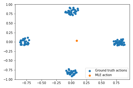
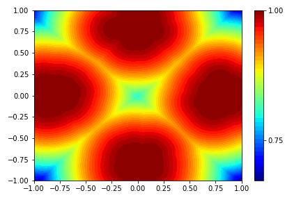
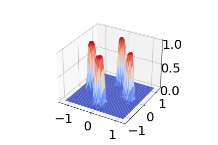
Below is a plot of the Morse density on a toy dataset. Note that this plots \(certainty = 1 - uncertainty\).

Part 2: Stable Reverse KL Constraint

Now we return to the basic BC constraint:

\[\pi_{BC} = argmin_\pi \mathbb{E}_{s, a \sim \mathcal{D}} [(\pi(s) - a)^2],\]

whose forward KL poses a problem when the underlying behavior policy is not unimodal. Instead, look at the uncertainty-minimizing constrained problem:

\[\pi_{BC} = argmin_\pi \mathbb{E}_{s, a \sim \mathcal{D}} [C^\pi(s, a) + \mu(\pi(s) - a)],\]

which minimizes uncertainty (\(C^\pi(s, a)\), I’ll get to what exactly this term is in a bit) and BC error.

At a glance, this objective does not make sense: surely minimizing uncertainty is equivalent to minimizing BC?

Well, nearly. They are equivalent when the behavior policy is unimodal, but, in a mixture behavior policy dataset, uncertainty minimization is mode-seeking.

This is still an ugly problem, but using the trickery behind weighted BC, we can obtain a cleaner policy objective:

\[argmin_\pi \mathbb{E}_{s, a \sim \mathcal{D}} [ (\pi(s) - a)^2 e^{\frac{1}{\mu} C^{\pi}(s, a)}] \Longleftrightarrow argmin_\pi D_{KL} (\pi || \pi_\beta),\]

where the final equivalence is exact when training a stochastic policy with entropy regularization.

In the paper, \(C^\pi(s, a) = certainty\) from the Morse net model. As certainty is bounded, the limits of the exponential certainty are \(1 \leq exp(certainty) \leq e^{1/\mu}\) and we can see this as a dynamic weight applied to the BC constraint: \(\omega(s, a) (\pi(s) - a)^2\). When the policy is out-of-distribution, \(\omega(s, a)\) is large leading to a strong pull towards an in-distribution action. In practice, we use \(\omega(s, a) = e^{\frac{1}{\mu} C^{\pi}(s, a)} - 1\) as this constraint coefficient must decay to zero for in-distribution actions (i.e. no pull when fully in distribution).

Finally, we plug replace TD3+BC’s minimalist constraint with this new dynamic constraint:

\[\pi^* = argmax_{\pi} \mathbb{E}_{s, a \sim \mathcal{D}} [Q(s, \pi(s)) - \omega(s, a) (\pi(s) - a)^2 ].\]

The Benefits

The paper evaluates the new constrained objective on various datasets and performs ablations. Advantages can be summarized as:

1. SOTA: TD3-BST performs extremely well, especially on the challenging Antmaze tasks which TD3+BC struggles in
2. Tuning: TD3-BST introduces two new hyperparameters, one more than TD3+BC, but retains the ease of tuning with hyperparameter values generalizing well across like tasks
3. Pluggable: Any weighted BC policy improvement objective can be replaced with BST and demonstrate better performance

The Drawbacks

Some drawbacks I see in practice are:

1. Morse network: this is yet another model to train, and as an empirical estimate of the behavior policy, is subject to estimation errors and will inevitably be sensitive to architecture, especially when moving beyond proprioceptive domains
2. Limited: this approach is designed using the properties of the Morse network in mind. Replacing the Morse net with almost any other uncertainty estimator will require careful tuning
3. Difficult to extend: in internal experiments, I tried and failed to apply BST to stochastic policies. For now, performance seems limited to deterministic policies - maybe someone with both compute and time may find it interesting to apply BST to SAC.